【Matplotlib】Python Format文~必要なものだけ厳選(理系)
こんにちは!
今回は、pythonでよく用いるformat文についてです
使い方
基本的な使い方は簡単です。
"{}"の中身を.format()で書き入れましょう
"{}".format(2019)
>>>'2019'
1つだけではなく、複数の文字や数を入れられます。
0番から始まる連番で指定すると、その数が入ります。
"I'm {0} {1}.".format("Noah", "Saito")
>>>"I'm Noah Saito."
具体例
次によく使うものを具体例で見ていきましょう。
小数点
小数点は「f」で表現します。fの前に何桁か指定できます。デフォルトは6桁です。
a = 0.2183
"{0:f} || {0:.1f}".format(a)
>>>'0.218300 || 0.2'
同様に指数表記のEもできます。こちらもデフォルトは6桁です。eが大文字か小文字かも指定できます。
a = 0.2183
"{0:e} || {0:.1e} || {0:.1E}".format(a)
>>>'2.183000e-01 || 2.2e-01 || 2.2E-01'
日にち
それぞれの日付のデータを使って以下のように表すことができます。
year, month, day = 2019, 1, 1
"{0}-{1}-{2}".format(year, month, day)
>>>'2019-1-1'
日付を'2019-01-01'のような桁数指定をしたい場合は、以下のように
「位置:0+桁数d」としましょう。(dは10整数である)
year, month, day = 2019, 1, 1
"{0:04d}-{1:02d}-{2:02d}".format(year, month, day)
>>>'2019-01-01'
さらに、モジュールのdatetimeを用いて表現できます。
import datetime
time = datetime.datetime(2019, 1, 1, 1, 1, 30)
"{:%Y-%m-%d %H:%M:%S}".format(time)
'2019-01-01 01:01:30'
ちなみに、月をJan, Feb...のようにしたい場合は、「%b」と指定します。
import datetime
for i in range(12):
    time = datetime.datetime(2019, i+1, 1)
    print("{:%b}".format(time))
>>>Jan Feb Mar Apr May Jun Jul Aug Sep Oct Nov Dec
n進数
2進数(binary number)、8進数(octal number)、10進数(decimal number)、16進数(hexadecimal number)があります。
binary, octal, decimal, hexadecimal = 30, 30, 30, 30
"{0:b}-{1:o}-{2:d}-{3:x}(or{3:X})".format(binary, octal, decimal, hexadecimal)
>>>'11110-36-30-1e(or1E)'
%
最後にパーセント表示です。100倍されることに注意してください。
そして、桁数も変更できます。デフォルトは6桁です。
a = 0.2183
"{0:%} || {0:.0%} || {0:.2%}".format(a)
>>>'21.830000% || 22% || 21.83%'
さらに詳しく
今回の記事はこちらを参考にして、理系が用いるものを厳選して紹介しました。
それでは
【Numpy&Matplotlib】 Python 軸を日付フォーマットに変更
こんにちは今日はx軸を日にちのフォーマットに変更する方法です。
DataFlame
まずは使用するデータフレームをファイルから読み込んでください。
今回私は適当に作成したデータを使います。
print(df)| Year | Month | Day | Hour | Minute | Data | |
|---|---|---|---|---|---|---|
| 0 | 2019 | 1 | 1 | 0 | 1 | 1.683375 |
| 1 | 2019 | 1 | 1 | 0 | 6 | 1.732797 |
| 2 | 2019 | 1 | 1 | 0 | 11 | 0.985744 |
| 3 | 2019 | 1 | 1 | 0 | 16 | 1.522657 |
| 4 | 2019 | 1 | 1 | 0 | 21 | 0.726131 |
| ... | ... | ... | ... | ... | ... | ... |
| 105115 | 2019 | 12 | 31 | 23 | 36 | 1.442926 |
| 105116 | 2019 | 12 | 31 | 23 | 41 | 1.532434 |
| 105117 | 2019 | 12 | 31 | 23 | 46 | 1.513058 |
| 105118 | 2019 | 12 | 31 | 23 | 51 | 0.594683 |
| 105119 | 2019 | 12 | 31 | 23 | 56 | 0.767968 |
105120 rows × 6 columns
1日当たりのDataの平均値を時系列プロットしてみます
#日平均
import calendar
xdata = []
year=2019
for j in range(12):
    month=j+1
    x=calendar.monthrange(year, month)[1] #*1
    df2 = df.loc[df["Month"]==month]
    for i in range(x):
        day = i + 1
        xdata0 = df2.loc[df2["Day"]==day]["Data"].mean()
        xdata.append(xdata0)
Keys
1) year年month月の日数を取ることができる。
例えばyear=2019 month=1 の時、x=31となる。
それではグラフを書いてみます。横軸はDN(Day Number)です。
import matplotlib.pyplot as plt
#グラフ作成
fig = plt.figure(figsize=(20,5))
plt.rcParams["font.size"] = 16
ax = plt.subplot(111)

ax.plot(np.arange(1,366), xdata)

ax.set_xlabel("DN")
ax.set_ylabel("Data")

ax.set_xlim(0,365)

plt.show()

fig.savefig("XXX.png",format="png", dpi=330)

DN⇒Datetime
次に横軸を日付にします。
time = []
year = 2019
for i in range(12):
    month = i + 1
    x=calendar.monthrange(year, month)[1]
    for j in range(x):
        day = j + 1
        t = "{0:04d}-{1:02d}-{2:02d}".format(year, month, day) #1*
        time.append(pd.to_datetime(t)) #*2
Keys
1) format文⇓
2)pd.to_datetime("2019-01-01 01:30:00:00")⇒Timestamp("2019-01-01 01:30:00:00")
オブジェクト⇒datetimeに変換されます
グラフ
#データの選択
x = time
y = xdata

#グラフ作成
fig = plt.figure(figsize=(20,5))
plt.rcParams["font.size"] = 16
ax = plt.subplot(111)

ax.plot(x, y)

#ラベル設定
ax.set_title(" ")
ax.set_ylabel("data")
ax.set_xlabel("Time")

#軸の設定 *1
ax.minorticks_on()
ax.tick_params(axis="both", which="major",direction="in",length=7,width=2,top="on",right="on")
ax.tick_params(axis="both", which="minor",direction="in",length=4,width=1,top="on",right="on")
ax.xaxis.set_major_formatter(DateFormatter("%b-%d"))
ax.xaxis.set_major_locator(mdates.MonthLocator(interval=2))
ax.xaxis.set_minor_locator(mdates.MonthLocator(interval=1))

#範囲設定
ax.set_xlim(datetime.datetime(2019, 1, 1), datetime.datetime(2019, 12, 31))

plt.show()

fig.savefig("XXX.png",format="png", dpi=330)

Keys
1)軸の設定
それでは 🌏
【Science】 Matplotlibで振り子ー二重振り子 カオスを知る
こんにちは!
今日は二重振り子でカオスを見てみたいと思います!
単振り子に基礎的なコードを載せています。
二重振り子
ドキュメント
モジュール
まずは必要なモジュールです。
import numpy as np
import matplotlib.pyplot as plt
import scipy.integrate as integrate
import matplotlib.animation as animation
軌跡
まずは二重振り子の軌跡を描いてみます。
%matplotlib nbagg
#物理量設定
G = 9.8 #重力加速度(m/s^2)
L1 = 1.0  #振り子(上)の長さ(m)
L2 = 1.0  #振り子(下)の長さ(m)
M1 = 1.0  #振り子(上)の重さ(kg)
M2 = 1.0  #振り子(下)の重さ(kg)


def derivs(state, t):

    dydx = np.zeros_like(state)
    dydx[0] = state[1]

    delta = state[2] - state[0]
    den1 = (M1+M2) * L1 - M2 * L1 * np.cos(delta) * np.cos(delta)
    dydx[1] = ((M2 * L1 * state[1] * state[1] * np.sin(delta) * np.cos(delta)
                + M2 * G * np.sin(state[2]) * np.cos(delta)
                + M2 * L2 * state[3] * state[3] * np.sin(delta)
                - (M1+M2) * G * np.sin(state[0]))
               / den1)

    dydx[2] = state[3]

    den2 = (L2/L1) * den1
    dydx[3] = ((- M2 * L2 * state[3] * state[3] * np.sin(delta) * np.cos(delta)
                + (M1+M2) * G * np.sin(state[0]) * np.cos(delta)
                - (M1+M2) * L1 * state[1] * state[1] * np.sin(delta)
                - (M1+M2) * G * np.sin(state[2]))
               / den2)

    return dydx

#初期値
dt = 0.05 #時間間隔
t = np.arange(0, 20, dt) #時間間隔分
th1 = 120.0 #振り子(上)初期角度
w1 = 0.0 #振り子(上)角速度
th2 = -10.0 #振り子(下)初期角度
w2 = 0.0 #振り子(下)角速度

state1 = np.radians([th1, w1, th2, w2]) # 初期状態

#微分方程式を解く
y01 = integrate.odeint(derivs, state1, t)


x1 = L1 * np.sin(y01[:, 0])
y1 = -L1 * np.cos(y01[:, 0])
x2 = L2 * np.sin(y01[:, 2]) + x1
y2 = -L2 * np.cos(y01[:, 2]) + y1

#--------------------グラフ-----------------------
fig = plt.figure()
ax = fig.add_subplot(111, autoscale_on=False, xlim=(-2, 2), ylim=(-2, 2))
ax.set_aspect("equal")
ax.grid()

line, = ax.plot([], [], "o-", lw=2)
locus, = ax.plot([], [], "r-", linewidth=2) #軌跡用
time_template = "time = %.1fs"
time_text = ax.text(0.05, 0.9, "", transform=ax.transAxes)

xlocus, ylocus = [], []
def init():
    line.set_data([], [])
    locus.set_data([], [])
    time_text.set_text("")
    return line,locus, time_text


def animate(i):
    thisx1 = [0, x1[i], x2[i]]
    thisy1 = [0, y1[i], y2[i]]
    xlocus.append(x2[i])
    ylocus.append(y2[i])

    line.set_data(thisx1, thisy1)
    locus.set_data(xlocus, ylocus)
    time_text.set_text(time_template % (i*dt))
    return line,locus, time_text


ani = animation.FuncAnimation(fig, animate, range(1, len(y01)),
                              interval=dt*1000, blit=True, init_func=init)
plt.show()
# ani.save("XXX.gif", writer="pillow", fps=20)
2個
次にいきなり複数の振り子にいくのはなんなので、2つの振り子を描写してみます。
%matplotlib nbagg
#物理量設定
G = 9.8 #重力加速度(m/s^2)
L1 = 1.0  #振り子(上)の長さ(m)
L2 = 1.0  #振り子(下)の長さ(m)
M1 = 1.0  #振り子(上)の重さ(kg)
M2 = 1.0  #振り子(下)の重さ(kg)


def derivs(state, t):

    dydx = np.zeros_like(state)
    dydx[0] = state[1]

    delta = state[2] - state[0]
    den1 = (M1+M2) * L1 - M2 * L1 * np.cos(delta) * np.cos(delta)
    dydx[1] = ((M2 * L1 * state[1] * state[1] * np.sin(delta) * np.cos(delta)
                + M2 * G * np.sin(state[2]) * np.cos(delta)
                + M2 * L2 * state[3] * state[3] * np.sin(delta)
                - (M1+M2) * G * np.sin(state[0]))
               / den1)

    dydx[2] = state[3]

    den2 = (L2/L1) * den1
    dydx[3] = ((- M2 * L2 * state[3] * state[3] * np.sin(delta) * np.cos(delta)
                + (M1+M2) * G * np.sin(state[0]) * np.cos(delta)
                - (M1+M2) * L1 * state[1] * state[1] * np.sin(delta)
                - (M1+M2) * G * np.sin(state[2]))
               / den2)

    return dydx

dt = 0.05
t = np.arange(0, 20, dt)

th1 = 120.0
th12 = 120.1
w1 = 0.0
th2 = -10.0
w2 = 0.0

#初期状態
state1 = np.radians([th1, w1, th2, w2])
state2 = np.radians([th12, w1, th2, w2])

#微分方程式を解く
y01 = integrate.odeint(derivs, state1, t)
y02 = integrate.odeint(derivs, state2, t)

x1 = L1 * np.sin(y01[:, 0])
y1 = -L1 * np.cos(y01[:, 0])
x2 = L2 * np.sin(y01[:, 2]) + x1
y2 = -L2 * np.cos(y01[:, 2]) + y1

x3 = L1 * np.sin(y02[:, 0])
y3 = -L1 * np.cos(y02[:, 0])
x4 = L2 * np.sin(y02[:, 2]) + x3
y4 = -L2 * np.cos(y02[:, 2]) + y3

fig = plt.figure()
ax = fig.add_subplot(111, autoscale_on=False, xlim=(-2, 2), ylim=(-2, 2))
ax.set_aspect("equal")
ax.grid()

line, = ax.plot([], [], "o-", lw=2)
line2, = ax.plot([], [], "o-", lw=2)
time_template = "time = %.1fs"
time_text = ax.text(0.05, 0.9, "", transform=ax.transAxes)


def init():
    line.set_data([], [])
    line2.set_data([], [])
    time_text.set_text("")
    return line,line2, time_text


def animate(i):
    thisx1 = [0, x1[i], x2[i]]
    thisy1 = [0, y1[i], y2[i]]
    thisx2 = [0, x3[i], x4[i]]
    thisy2 = [0, y3[i], y4[i]]

    line.set_data(thisx1, thisy1)
    line2.set_data(thisx2, thisy2)
    time_text.set_text(time_template % (i*dt))
    return line,line2, time_text


ani = animation.FuncAnimation(fig, animate, range(1, len(y01)),
                              interval=dt*1000, blit=True, init_func=init)
plt.show()
#ani.save("XXX.gif", writer="pillow", fps=20)
カオス
最後にカオスを描写してみます。
先ほどよりも振り子数が一気に増えます。
%matplotlib nbagg
#物理量設定
G = 9.8 #重力加速度(m/s^2)
L1 = 1.0  #振り子(上)の長さ(m)
L2 = 1.0  #振り子(下)の長さ(m)
M1 = 1.0  #振り子(上)の重さ(kg)
M2 = 1.0  #振り子(下)の重さ(kg)


def derivs(state, t):

    dydx = np.zeros_like(state)
    dydx[0] = state[1]

    delta = state[2] - state[0]
    den1 = (M1+M2) * L1 - M2 * L1 * np.cos(delta) * np.cos(delta)
    dydx[1] = ((M2 * L1 * state[1] * state[1] * np.sin(delta) * np.cos(delta)
                + M2 * G * np.sin(state[2]) * np.cos(delta)
                + M2 * L2 * state[3] * state[3] * np.sin(delta)
                - (M1+M2) * G * np.sin(state[0]))
               / den1)

    dydx[2] = state[3]

    den2 = (L2/L1) * den1
    dydx[3] = ((- M2 * L2 * state[3] * state[3] * np.sin(delta) * np.cos(delta)
                + (M1+M2) * G * np.sin(state[0]) * np.cos(delta)
                - (M1+M2) * L1 * state[1] * state[1] * np.sin(delta)
                - (M1+M2) * G * np.sin(state[2]))
               / den2)

    return dydx

dt = 0.05
t = np.arange(0, 20, dt)


th1s = np.arange(120.0,120.01,0.0001)
w1 = 0.0
th2 = -10.0
w2 = 0.0


#初期状態
states=[]
for th1 in th1s:
    state = np.radians([th1, w1, th2, w2])
    states.append(state)

#微分方程式を解く
ys=[]
for state in states:
    y = integrate.odeint(derivs, state, t)
    ys.append(y)

x1s,x2s,y1s,y2s=[],[],[],[]
for y in ys:
    x1 = L1 * np.sin(y[:, 0])
    y1 = -L1 * np.cos(y[:, 0])
    x2 = L2 * np.sin(y[:, 2]) + x1
    y2 = -L2 * np.cos(y[:, 2]) + y1
    x1s.append(x1)
    y1s.append(y1)
    x2s.append(x2)
    y2s.append(y2)

fig = plt.figure()
ax = fig.add_subplot(111, autoscale_on=False, xlim=(-2, 2), ylim=(-2, 2))
ax.set_aspect("equal")
ax.grid()

lines=[]
for i in range(len(th1s)):
    line, = ax.plot([], [], "o-", lw=2)
    lines.append(line,)
time_template = "time = %.1fs"
time_text = ax.text(0.05, 0.9, "", transform=ax.transAxes)


def init():
    for line in lines:
        line.set_data([], [])
    time_text.set_text('')
    return lines, time_text


def animate(i):
    for j in range(len(lines)):
        line = lines[j]
        thisx1 = [0, x1s[j][i], x2s[j][i]]
        thisy1 = [0, y1s[j][i], y2s[j][i]]

        line.set_data(thisx1, thisy1)
    time_text.set_text(time_template % (i*dt))
    return lines, time_text


ani = animation.FuncAnimation(fig, animate, range(1, len(y)),
                              interval=dt*1000, blit=True, init_func=init)
plt.show()

# ani.save("XXX.gif", writer="pillow", fps=20)
それでは🌏
【Science】 Matplotlibで振り子ー単振り子
こんにちは
今日は関数を使って、単振り子をアニメーションを作成したいと思います!
アニメーションの基礎は前の記事を参照してください!
微分方程式
単振り子を描写するのに関数が必要なので書き方を確認しましょう
モジュール
from scipy.integrate import solve_ivp
import matplotlib.pyplot as plt
import numpy as np
解く
それでは、solve_ivpで指数関数的減衰を解いてみます。
指数関数的減衰は半減期の計算で使われますね
https://www.nli-research.co.jp/report/detail/id=58700?site=nli
# 指数関数的減衰
def exponential_decay(t, y):
    return -0.5 * y

t_span = [0, 10] #tの範囲
y0 = [2, 4, 8] #y初期値
t_eval = np.arange(t_span[0], t_span[-1], 0.1) #tの間隔
sol = solve_ivp(exponential_decay, t_span, y0, t_eval=t_eval) #方程式を解く
解(sol)の中身を確認します。
print(sol.t)
⇒[0. 0.1 0.2 0.3…9.7 9.8 9.9]
print(sol.y)
⇒[[2. 1.90245885 1.809668…0.01492886 0.01420166]
 [4. 3.8049177 3.619336…0.02985772 0.02840332]
 [8. 7.6098354 7.238672…0.05971543 0.05680663]]
tに対するyが作成されていることがわかります。
描写
それでは描写してみます
fig, ax = plt.subplots()
ax.plot(sol.t, sol.y[0])
ax.plot(sol.t, sol.y[1])
ax.plot(sol.t, sol.y[2])

ax.set_xlabel("T")
ax.set_ylabel("Y-axis")

ax.set_xlim(t_span[0],t_span[-1])
ax.set_ylim(0, 9)

plt.show()

#保存
#fig.savefig("XXX.png", format="png", dpi=330)

単振り子
それでは単振り子のアニメーション作成してみます。
以下を参考に作成しました。
モジュール
まずはモジュールをインポートします
from scipy.integrate import solve_ivp
from matplotlib.animation import FuncAnimation
import matplotlib.pyplot as plt
import numpy as np
単振り子
%matplotlib nbagg
G = 9.8  # 重力加速度(m/s^2)
L = 1.0  # 振り子の長さ(m)

# 運動方程式を解く
def eom(t, state):
    dydt = np.zeros_like(state)
    dydt[0] = state[1]
    dydt[1] = -(G/L)*np.sin(state[0])
    return dydt

#設定
t_span = [0,20] #時間 (s)
dt = 0.05# 時間の間隔 (s)
t = np.arange(t_span[0], t_span[-1], dt)# 時間の間隔のarray作成

#初期状態設定
th1 = 45.0# 角度 [deg]
w1 = 0.0 # 初期角速度 [deg/s]
state = np.radians([th1, w1])# 初期状態

#微分方程式を解く
sol = solve_ivp(eom, t_span, state, t_eval=t)
theta = sol.y[0] #y[0]=θ、y[1]=ω

x = L * np.sin(theta)
y = -L * np.cos(theta)

#ーーーーーーグラフーーーーーーー
fig, ax = plt.subplots()

line, = ax.plot([], [], "o-", linewidth=2)
time_template = "time = %.1fs"
time_text = ax.text(0.05, 0.9, " ", transform=ax.transAxes)

def init():
    line.set_data([], [])
    time_text.set_text("")
    return line, time_text

def animate(i):
    thisx = [0, x[i]]
    thisy = [0, y[i]]
    line.set_data(thisx, thisy)
    time_text.set_text(time_template % (i*dt))
    return line, time_text


ani = FuncAnimation(fig, animate, frames=np.arange(0, len(t))
                    , interval=25, blit=True,init_func=init)

ax.set_xlim(-L-0.5,L+0.5)
ax.set_ylim(-L-0.5,L+0.5)
ax.set_aspect("equal")
ax.grid()

plt.show()

#ani.save("XXX.gif", writer="pillow", fps=20)
時間変化
次に単振り子の角度、x, yの時間変化をプロットしてみます
fig = plt.figure(figsize=(10,5))
ax1 = plt.subplot(111)
ax2 = ax1.twinx()

ax1.plot(sol.t, sol.y[0], label="$\\theta$")
ax2.plot(sol.t, x , color="r", linestyle="--",label="x")
ax2.plot(sol.t, y , color="g", linestyle="--",label="y")

ax1.set_yticks(np.array([-np.pi, -(1/3)*np.pi, -(1/4)*np.pi, -(1/6)*np.pi, 0,(1/6)*np.pi,(1/4)*np.pi,(1/3)*np.pi,np.pi]))
ax1.set_yticklabels(["-$\pi$","-1/3$\pi$","-1/4$\pi$","-1/6$\pi$", "0","1/6$\pi$","1/4$\pi$","1/3$\pi$","$\pi$"])
ax1.set_ylabel("$\\theta$")
ax2.set_yticks(np.array([-1,-(1/2)*np.sqrt(3),-(1/2)*np.sqrt(2),-(1/2)*np.sqrt(1),0,(1/2)*np.sqrt(1),(1/2)*np.sqrt(2),(1/2)*np.sqrt(3),1]))
ax2.set_yticklabels(["$-$1","$-\sqrt{\\frac{3}{2}}$","$-\sqrt{\\frac{2}{2}}$","$-{\\frac{1}{2}}$", "0","${\\frac{1}{2}}$","$\sqrt{\\frac{2}{2}}$","$\sqrt{\\frac{3}{2}}$","1"])
ax2.set_ylabel("X, Y")
ax1.set_xlabel("T")

ax1.set_xlim(t_span[0],t_span[-1])
ax1.set_ylim(-(1/3)*np.pi,(1/3)*np.pi)

#凡例
h1, l1 = ax1.get_legend_handles_labels()
h2, l2 = ax2.get_legend_handles_labels()
ax1.legend(h1+h2, l1+l2, ncol=3, fontsize=12)

plt.show()

#保存
#fig.savefig("XXX.png", format="png", dpi=330)

単振り子の軌跡
%matplotlib nbagg
G = 9.8  # 重力加速度(m/s^2)
L = 1.0  # 振り子の長さ(m)

# 運動方程式を解く
def eom(t, state):
    dydt = np.zeros_like(state)
    dydt[0] = state[1]
    dydt[1] = -(G/L)*np.sin(state[0])
    return dydt

#設定
t_span = [0,20] #時間 (s)
dt = 0.05# 時間の間隔 (s)
t = np.arange(t_span[0], t_span[-1], dt)# 時間の間隔のarray作成

#初期状態設定
th1 = 45.0# 角度 [deg]
w1 = 0.0 # 初期角速度 [deg/s]
state = np.radians([th1, w1])# 初期状態

#微分方程式を解く
sol = solve_ivp(eom, t_span, state, t_eval=t)
theta = sol.y[0] #y[0]=θ、y[1]=ω

x = L * np.sin(theta)
y = -L * np.cos(theta)

#ーーーーーーグラフーーーーーーー
fig, ax = plt.subplots()

line, = ax.plot([], [], "o-", linewidth=2)
locus, = ax.plot([], [], 'r-', linewidth=2)
xlocus, ylocus = [], []
time_template = "time = %.1fs"
time_text = ax.text(0.05, 0.9, " ", transform=ax.transAxes)


def init():
    line.set_data([], [])
    time_text.set_text("")
    return line, time_text

def animate(i):
    thisx = [0, x[i]]
    thisy = [0, y[i]]
    line.set_data(thisx, thisy)
    xlocus.append(x[i])
    ylocus.append(y[i])

    locus.set_data(xlocus, ylocus)
    time_text.set_text(time_template % (i*dt))
    return line,xlocus, ylocus, time_text


ani = FuncAnimation(fig, animate, frames=np.arange(0, len(t))
                    , interval=25, blit=True,init_func=init)

ax.set_xlim(-L-0.5,L+0.5)
ax.set_ylim(-L-0.5,L+0.5)
ax.set_aspect("equal")
ax.grid()

plt.show()

#ani.save("XXX.gif", writer="pillow", fps=20)
複数の単振り子
次に複数の単振り子です。
%matplotlib nbagg
G = 9.8  # 重力加速度(m/s^2)
L = 1.0  # 振り子の長さ(m)

# 運動方程式を解く
def eom(t, state):
    dydt = np.zeros_like(state)
    dydt[0] = state[1]
    dydt[1] = -(G/L)*np.sin(state[0])
    return dydt

#設定
t_span = [0,20] #時間 (s)
dt = 0.05# 時間の間隔 (s)
t = np.arange(t_span[0], t_span[-1], dt)# 時間の間隔のarray作成

#初期状態設定

th1s = np.arange(40.0,90.0,10.0)
w1 = 0.0 # 初期角速度 [deg/s]

states=[]
for th1 in th1s:
    state = np.radians([th1, w1])# 初期状態
    states.append(state)

thetas=[]
for state in states:
    sol = solve_ivp(eom, t_span, state, t_eval=t)
    theta = sol.y[0] #y[0]=θ、y[1]=ω
    thetas.append(theta)

xs,ys=[],[]
for theta in thetas:
    x = L * np.sin(theta)
    y = -L * np.cos(theta)
    xs.append(x)
    ys.append(y)


#ーーーーーーグラフーーーーーーー
fig, ax = plt.subplots()

lines=[]
for i in range(len(th1s)):
    line, = ax.plot([], [], 'o-', lw=2, label=th1s[i])
    lines.append(line,)

time_template = "time = %.1fs"
time_text = ax.text(0.05, 0.9, " ", transform=ax.transAxes)


def init():
    for line in lines:
        line.set_data([], [])
    time_text.set_text("")
    return line, time_text

def animate(i):
    for j in range(len(lines)):
        line = lines[j]
        thisx = [0, xs[j][i]]
        thisy = [0, ys[j][i]]
        line.set_data(thisx, thisy)

    time_text.set_text(time_template % (i*dt))
    return line, time_text


ani = FuncAnimation(fig, animate, frames=np.arange(0, len(t))
                    , interval=25, blit=True,init_func=init)

ax.set_xlim(-L-0.5,L+0.5)
ax.set_ylim(-L-0.5,L+0.5)
ax.legend(title="init $\\theta$")
ax.set_aspect("equal")
ax.grid()

plt.show()

3ani.save("XXX.gif", writer="pillow", fps=20)
次は二重振り子によるカオスをアニメーションで描写したいと思います!
それでは🌏
【Matplotlib】アニメーション(FuncAnimation)
こんにちは
今日はMatplotlibのFuncAnimationを使ってアニメーションを作成したいと思います。
グラフ作成
Step1
まずはドキュメントの3個目のsin関数を描写してみましょう。
Step2
ドキュメントを参考にして
「y=ax²」のグラフを描いてみます。
モジュール
import numpy as np
import matplotlib.pyplot as plt
from matplotlib.animation import FuncAnimation
グラフ
%matplotlib nbagg
fig, ax = plt.subplots()
#y = ax^2
xdata, ydata = [], []
line, = plt.plot([], [], "b-") #*1
a = 1/2

def init():
    ax.set_title("Basic")

    ax.set_xlim(-10,10)
    ax.set_ylim(-100,100)
    #*2
    ax.axhline(y=0, xmin=-10, xmax=10, color="k", linestyle="--")
    ax.axvline(x=0, ymin=-100, ymax=100, color="k", linestyle="--")

    ax.set_xlabel("X")
    ax.set_ylabel("Y")
    ax.grid() #*3

    return line,

def update(frame):
    #y=ax^2
    xdata.append(frame)
    ydata.append(a*(frame)*(frame))
    line.set_data(xdata, ydata)

    return line,

ani = FuncAnimation(fig, update, frames=np.linspace(-10, 10, 40),
                    init_func=init, blit=True) #*4
plt.show()

#ani.save("XXX.gif", writer="pillow", fps=15)

Keys
1) "b-"⇒colorが「b(blue)」でlineが「-」です
2) axhline(y=Y, xmin=最小値, xmax=最大値)⇒y=Yで直線を引く
axvline(x=X, ymin=最小値, ymax=最大値)⇒x=Xで直線を引く
3) 図にグリッド欄を拭く
4) np.linspace(a, b, n)⇒初項a、末項bで、項数nの等差数列を作成
(e.g.)

np.linspace(0,20,20)
⇒array([ 0. , 1.05263158, 2.10526316, 3.15789474, 4.21052632,
 5.26315789, 6.31578947, 7.36842105, 8.42105263, 9.47368421,
 10.52631579, 11.57894737, 12.63157895, 13.68421053, 14.73684211,
 15.78947368, 16.84210526, 17.89473684, 18.94736842, 20. ])
Step3
最後に複数の線をプロットしてみます
モジュール
import numpy as np
import matplotlib.pyplot as plt
from matplotlib.animation import FuncAnimation
グラフ
%matplotlib nbagg

fig, ax = plt.subplots()
#sin
xdata, ydata = [], []
ln, = plt.plot([], [], "b-")
#cos
xdata2, ydata2 = [], []
ln2, = plt.plot([], [], "r-")
#tan
xdata3, ydata3 = [], []
ln3, = plt.plot([], [], "go",alpha=0.5)

def init():
    ax.set_title("SIN & COS & TAN")

    ax.set_xlim(-2*np.pi, 2*np.pi)
    ax.set_ylim(-1, 1)
    ax.axhline(y=0, xmin=-2*np.pi, xmax=2*np.pi, color="k", linestyle="--")
    ax.axvline(x=0, ymin=-1, ymax=1, color="k", linestyle="--")

    ax.set_xticks(np.arange(-2*np.pi,2*np.pi+0.01,(1/2)*np.pi)) #*2
    ax.set_xticklabels(["-2$\pi$","-3/2$\pi$","-$\pi$","-1/2$\pi$", "0","1/2$\pi$","$\pi$","3/2$\pi$", "2$\pi$"]) #*1, 2
    ax.set_xlabel("$\\theta$") #*2
    ax.grid()

    return ln,

def update(frame):
    #sin
    xdata.append(frame)
    ydata.append(np.sin(frame))
    ln.set_data(xdata, ydata)
    #cos
    xdata2.append(frame)
    ydata2.append(np.cos(frame))
    ln2.set_data(xdata2, ydata2)
    #tan
    xdata3.append(frame)
    ydata3.append(np.tan(frame))
    ln3.set_data(xdata3, ydata3)

    return ln,ln2,ln3

ani = FuncAnimation(fig, update, frames=np.linspace(-2*np.pi, 2*np.pi, 300),
                    init_func=init, blit=True)
plt.show()

# ani.save("XXX.gif", writer="pillow", fps=15)

Keys
1)ラベルをラジアンに変換
2)ギリシャ文字
いかがだったでしょうか。
それでは🌏
【Matplotlib】2軸のグラフを作成しよう
こんにちは!2軸のグラフ作成をします
データの用意ができていて、図の書き方だけ知りたいという方は、描写 2軸へ!!
モジュール
必要なモジュールをインポートします
import numpy as np
import matplotlib.pyplot as plt
データ
それではまず初めにデータを用意します。
今回はランダムなデータを使用します。
x = np.arange(0,100,1)
y1 = np.random.rand(100)
y2 = np.random.rand(100) * 100
描写
1軸
2軸の描写の前に、それぞれのデータをプロットして確認しておきましょう。
fig = plt.figure(figsize=(10, 5))
plt.rcParams["font.size"] = 18 #fontsize一括設定
ax1 = plt.subplot(211)
ax2 = plt.subplot(212)

ax1.plot(x, y1)
ax2.plot(x, y2)

#軸設定
ax1.set_ylabel("Y1-axis")
ax2.set_ylabel("Y2-axis")
ax1.label_outer()

plt.show()
#保存
fig.savefig("XXX.png" ,format="png", dpi=330) 
2軸
それでは本題の2軸グラフです。
今回の目的は2軸グラフの描写なので、細かい設定はしません。
fig = plt.figure(figsize=(10, 3))
plt.rcParams["font.size"] = 18
ax1 = plt.subplot(111)
ax2 = ax1.twinx() #*1

ax1.plot(x, y1, color="b", label = "Y1")
ax2.plot(x, y2, color="r", label = "Y2")

#軸設定
ax1.set_ylabel("Y1-axis")
ax2.set_ylabel("Y2-axis")
#範囲設定
ax1.set_xlim(0,100)
ax1.set_ylim(0,1.2)
ax2.set_ylim(0,120)

#*2
h1, l1 = ax1.get_legend_handles_labels()
h2, l2 = ax2.get_legend_handles_labels()
ax1.legend(h1+h2, l1+l2, ncol=2, fontsize=12)

plt.show()

fig.savefig("XXX.png" ,format="png", dpi=330)

Keys
1) ax2は、ax1に.twinx()で結合します
2)凡例(legend)の表示です。
通常に
ax1.legend()
ax2.legend()
としても良いのですが、それぞれが独立してしまうため表示が不自然になります。
したがって、.get_legend_handles_labels()から得られたhとlを足し算することによって統一の凡例が表示できます。
参考
ちなみにbarで違うデータを表示させると以下のようになります。
このようにすると、2つのデータの対比がしやすくなりますね!

それでは 🌏
【Science】水平線までどのくらいの距離?Part2ーマップで表示
こんにちは!
前回に引き続き、Cartopyでマップに表示したいと思います
[前回の記事]
水平線までどのくらいの距離なのか?
今回はCartopyを使ってどこまで見られるのか表示してみました!
都道府県などの境を表示するためにGADMのシェープファイルを利用させていただきました。
[ シェープファイル利用(Japan⇒Shapefile)]
地図
大気スケール
まずは大気スケールです。
日本列島の端から端まではだいたい2000 kmです
したがって、半径が1000 kmだとだいたい日本列島全体が見れますね
飛行機の高度の10 kmくらいの時はいちばん小さい円です。
それでも関東地方全体は軽く眺められますね。

| スケール | H | D | |
| 名前 | m | km | |
| 大気 | 熱圏 | 10000 | 1133.23 |
| 中間層 | 8000 | 1012.8 | |
| 成層圏 | 5000 | 799.75 | |
| 対流圏 | 1000 | 357.099 | |
山スケール
次に山スケールです。
今回は富士山とエベレストのみにします。(他はそこまで高さが変わらないので)
赤の点は富士山頂です。
富士山とエベレストで見られる範囲を比べると100 km程しか変わらないのでそこまで違いが見られませんね。それにしても、山に登るだけでここまで見れるのはすごいですよね。

建物スケール
次に建物スケールです。
赤い点は東京スカイツリーです。(634 m)
世界1位のブルジュハリファとスカイツリーを比較してもあまり見える距離は変わらないんですね。意外です。
しかし、東京タワーと比べると差が大きくなりますね。
都内の大きな高層マンションでは水平距離で24区見れそうですね、障害物がなければですが(笑

| スケール | H | D | |
| 名前 | m | km | |
| 建物 | ブルジュ ハリファ | 828 | 102.7 |
| 東京スカイツリー | 634 | 89.9 | |
| 東京タワー | 333 | 65.1 | |
| 福岡タワー | 234 | 54.6 | |
| 40階 | 150 | 43.7 | |
| 20階 | 60 | 27.7 | |
| 10階 | 30 | 19.6 | |
| 5階 | 12 | 12.4 | |
| 3階 | 9 | 10.7 | |
| 2階 | 6 | 8.7 | |
人スケール
最後に人スケールです。
平均身長あたりだと150ー170 cmなので見られる距離は4キロほどです。
東京ディズニーリゾートのある舞浜からです。
実際東京湾に立つと、羽田空港から千葉県が見られますし、千葉県から東京や川崎が見られます。
それは、水平線ではなく建物の高さがあるためや地上の高低差ならびに大気の屈折があるためと考えられます。

| スケール | H | D | |
| 名前 | m | km | |
| 身長 | 10cm | 0.1 | 1.1 |
| 30cm | 0.3 | 2 | |
| 50cm | 0.5 | 2.5 | |
| 70cm | 0.7 | 3 | |
| 90cm | 0.9 | 3.4 | |
| 110cm | 1.1 | 0.7 | |
| 130cm | 1.3 | 4.1 | |
| 150cm | 1.5 | 4.4 | |
| 170cm | 1.7 | 4.7 | |
| 190cm | 1.9 | 4.9 | |
| 210cm | 2.1 | 5.2 | |
| 230cm | 2.3 | 5.4 | |
| 250cm | 2.5 | 5.6 | |
| 270cm | 2.7 | 5.9 |
コード
まずは描写に必要なモジュールをインポートします
import matplotlib.pyplot as plt
import cartopy.crs as ccrs
import cartopy.feature as cfeature
#shape file
import cartopy.io.shapereader as shpreader
次に、地球状のどこかかの点から円を描くので
半径(r km)と中心の緯度経度から、円の緯度経度座標に変換します
# 円
def circle(r,S,T):
    #r:radius(km), (S,T):centerDegree
    s,t = S*111, T*111
    points = 1000
    theta = np.linspace(0, 2 * np.pi, points)
    x = r * np.sin(theta) + s
    y = r * np.cos(theta) + t

    #x,y=>Degree
    X, Y = x/111, y/111
    return (X,Y)
Keys
「km⇄緯度経度」は赤道半径を利用した値で変換しました
km = Degree ✕ 111
それでは描写してみます
def main():
    fig = plt.figure(figsize=(5,5))
    plt.rcParams["font.size"] = 18
    # TokyoStation
    ts_lon = 139.767125
    ts_lat = 35.681236

    ax = fig.add_subplot(1,1,1, projection=ccrs.PlateCarree())
    ax.set_extent([ts_lon-1, ts_lon+1, ts_lat-1, ts_lat+1], crs=ccrs.PlateCarree())
    ax.set_title("Title")

    ax.add_feature(cfeature.BORDERS, linestyle=":")
    #都道府県境と市町村境
    fname1 = "data/gadm36_JPN_shp/gadm36_JPN_1.shp"
    fname2 = "data/gadm36_JPN_shp/gadm36_JPN_2.shp"
    adm1_shapes = list(shpreader.Reader(fname1).geometries())
    adm2_shapes = list(shpreader.Reader(fname2).geometries())

    #データのプロット
    ax.add_geometries(adm1_shapes, ccrs.PlateCarree(),
                  edgecolor="k",facecolor="w",alpha=0.5)
    ax.add_geometries(adm2_shapes, ccrs.PlateCarree(),
                  edgecolor="gray", facecolor="w",  alpha=0.5)

    #TokyoStation

    ax.scatter(ts_lon,ts_lat,s=20,c="r",alpha=1, zorder=10)
    c = circle(100, ts_lon,ts_lat)
    ax.plot(c[0],c[1],c="b",alpha=1, zorder=10)

    plt.show()

if __name__ == "__main__":
    main()
参考コード
それでは🌏
関連記事
【Science】水平線までどのくらいの距離?Part1
こんにちは!
皆さん水平線までの距離ってどのくらいなんだろうって考えたことありませんか?
今回はそれを計算してみました。
計算
半径をrとし、地表面からの高さをhとします。

そして地球(あるいは天体)を完全な球体と仮定し、hと円との接線を引き、そこまでの距離をdとします。三平方の定理より、
⇔
∵d>0
※簡易的な計算であるため、dまでには障害物がないと仮定し、大気による光の屈折はしないと仮定します。地域で気温や大気質に違いがあるため、考慮しないです。
※実際見える対象物は平面ではなく、高さがあるのでdまでが見える範囲とは限りません。
高さと距離の関係
試しにエベレストで距離dを調べてみました。エベレストの標高は8848 mですので、
地球の赤道半径6378 kmを利用すると、約340 kmでした。
意外と見れますね。
これを踏まえていろいろな高さから見られる距離を求めてみました。

グラフ
大気スケール
上から熱圏、中間層、成層圏、対流圏です。
高度が高くなればなるほど見える距離は大きくなりますが、その変化の幅は小さくなります。
それはdの式がh²のルートに比例するからでしょう。

山スケール
世界の山ランキングと日本の山ランキングからのデータをプロットしました。
世界トップ10の山はどれも8000 m級で、それほど差が無いので見える距離もほどんど変わらず、300ー350 km
日本のトップテンも同様に3000 m急なので、200 km
という結果になりました。

Highest Mountain Peaks of the World
建物スケール
次はさらに低い建物で見ていきます。
世界一のブルジュハリファだと102 m
日本一の東京スカイツリーだと90 m
でした。
他にも1階あたりを3 mとして、40 m, 20 m, 10m, 5m, 3m, 2mと計算してみました
人スケール
そして、身長によってどのくらい見える距離が変わるのかを調べてみました。
身長170 cmのとき4.7 km
身長150 cmのとき4.4 km
身長が20 cm違っても300 m位しか差がありませんね(笑

太陽系
先ほどまでは地球の半径で計算してきましたが、次に太陽系の惑星の半径で計算してみました。
高さは人スケールにしました。
太陽、水星、金星、地球、火星、木星、土星、天王星、海王星、冥王星、エリス、月
太陽は圧倒的に半径が大きいので差が明瞭に見られますね。

まとめ
人はだいたい4キロくらいですね
| スケール | H | D | スケール | H | D | ||
| 名前 | m | km | 名前 | m | km | ||
| 大気 | 熱圏 | 10000 | 1133.23 | 建物 | ブルジュ ハリファ | 828 | 102.7 |
| 中間層 | 8000 | 1012.8 | 東京スカイツリー | 634 | 89.9 | ||
| 成層圏 | 5000 | 799.75 | 東京タワー | 333 | 65.1 | ||
| 対流圏 | 1000 | 357.099 | 福岡タワー | 234 | 54.6 | ||
| 山(世界) | エベレスト | 8850 | 335.9 | 40階 | 150 | 43.7 | |
| K2 | 8611 | 331.4 | 20階 | 60 | 27.7 | ||
| カンチェンジュンガ | 8586 | 330.9 | 10階 | 30 | 19.6 | ||
| ローツェ | 8516 | 329.5 | 5階 | 12 | 12.4 | ||
| マカルー | 8463 | 328.5 | 3階 | 9 | 10.7 | ||
| チョ・オユ- | 8201 | 323.4 | 2階 | 6 | 8.7 | ||
| ダウラギリ | 8167 | 322.7 | 身長 | 10cm | 0.1 | 1.1 | |
| マナスル | 8163 | 322.6 | 30cm | 0.3 | 2 | ||
| ナンガ・パルバット | 8125 | 321.9 | 50cm | 0.5 | 2.5 | ||
| アンナプルナ | 8091 | 321.2 | 70cm | 0.7 | 3 | ||
| 山(日本) | 富士山 | 3776 | 219.4 | 90cm | 0.9 | 3.4 | |
| 北岳 | 3193 | 201.7 | 110cm | 1.1 | 0.7 | ||
| 奥穂高岳 | 3190 | 201.6 | 130cm | 1.3 | 4.1 | ||
| 間ノ岳 | 3190 | 201.6 | 150cm | 1.5 | 4.4 | ||
| 槍ヶ岳 | 3189 | 201.3 | 170cm | 1.7 | 4.7 | ||
| 東岳 | 3141 | 200.1 | 190cm | 1.9 | 4.9 | ||
| 赤石岳 | 3121 | 199.4 | 210cm | 2.1 | 5.2 | ||
| 涸沢岳 | 3110 | 199.1 | 230cm | 2.3 | 5.4 | ||
| 北穂高岳 | 3106 | 199 | 250cm | 2.5 | 5.6 | ||
| 大喰岳 | 3101 | 198.8 | 270cm | 2.7 | 5.9 | ||
是非皆さんも半径や高度を変えていろいろと調べてみてください!
それでは🌏
【Jupyter Notebook】記号
こんにちは!
科学(気象系)で主に使う記号を紹介します。
LaTeXと少し違って、「\」を2つ付けるものもあるので注意しましょう。
| Symbol_1 | Symbol_2 | ||||
| Symbol Name | Letter | Jupyter | Symbol Name | Letter | Jupyter |
| イコール | = | = | 大なり | > | > |
| ノットイコール | ≠ | $\\neq$ | 小なり | < | < |
| ニアリーイコール | ≃ | $\simeq$ | 十分大 | ≫ | $\gg$ |
| プラス | + | + | 十分小 | ≪ | $\ll$ |
| マイナス | - | $-$ | 以上 | ≥ | $\geq$ |
| 掛ける | × | $\\times$ | 以上 | ≧ | $\geqq$ |
| 割る | ÷ | $\div$ | 以下 | ≤ | $\leq$ |
| プラスマイナス | ± | $\pm$ | 以下 | ≦ | $\leqq$ |
| マイナスプラス | ∓ | $\mp$ | 無限 | ∞ | $\infty$ |

Keys
neq = not equal
simeq = similar equal
div = division
pm = plus minus
mp = minus plus
geq = greater or equal
leq = less or equal
infty = infinity
参考(LaTeX)
それでは🌏
類似記事
【Jupyter Notebook】ギリシャ文字
こんにちは
今回は、Jupyternotebookでグラフ作成時によく使う
ギリシャ文字についてです。
小文字のαやβなどの文字は、「\」を二つ(「\\」)付けないといけないので
注意しましょう。
| Capital | Small | |||
| Greek Alphabet | Letter | Jupyter | Letter | Jupyter |
| アルファ | Α | $A$ | α | $\\alpha$ |
| ベータ | B | $B$ | β | $\\beta$ |
| ガンマ | Γ | $\Gamma$ | γ | $\gamma$ |
| デルタ | Δ | $\Delta$ | δ | $\delta$ |
| イプシロン | Ε | $E$ | ε | $\epsilon$ |
| ゼータ | Z | $Z$ | ζ | $\zeta$ |
| エータ | Η | $H$ | η | $\eta$ |
| シータ | Θ | $\\Theta$ | θ | $\\theta$ |
| イオタ | Ι | $I$ | ι | $\iota$ |
| カッパ | Κ | $K$ | κ | $\kappa$ |
| ラムダ | Λ | $\Lambda$ | λ | $\lambda$ |
| ミュー | M | $M$ | μ | $\mu$ |
| ニュー | N | $N$ | ν | $\\nu$ |
| クサイ | Ξ | $\\Xi$ | ξ | $\\xi$ |
| オミクロン | Ο | $O$ | ο | $\o$ |
| パイ | Π | $\Pi$ | π | $\pi$ |
| ロー | Ρ | $P$ | ρ | $\\rho$ |
| シグマ | Σ | $\Sigma$ | σ | $\sigma$ |
| タウ | Τ | $T$ | τ | $\\tau$ |
| ウプシロン | Υ | $\\Upsilon$ | υ | $\\upsilon$ |
| ファイ | Φ | $\Phi$ | φ | $\phi$ |
| キー | Χ | $X$ | χ | $\chi$ |
| プサイ | Ψ | $\Psi$ | ψ | $\psi$ |
| オメガ | Ω | $\Omega$ | ω | $\omega$ |

参考
それでは🌏
類似記事
【Matplotlib】Gridspecーグラフの柔軟な分割(3:1でもで4:1でも)
こんにちは。
グラフの分割をすると思うのですが、普通に分割すると1:1とか一つ一つが同じ大きさのグラフになりますよね。
そこで今回はMatplotlibのGridspecを用いて、3:1やさらに複雑なグラフの分割をしていきたいと思います!
★事前に必要な知識
グラフの基本的な書き方(matplotlib)
リストのスライス
基礎
まずは今回使うGridspecをインポートしましょう・
import matplotlib.pyplot as plt
from matplotlib import gridspec
例1
縦方向に3:1で分割してみます
fig = plt.figure(figsize=(4,3))
#分割 *1
ncols=2
nrows=1
gs = gridspec.GridSpec(ncols, nrows, height_ratios=(3, 1))
ax1 =  fig.add_subplot(gs[:1, 0])
ax2 =  fig.add_subplot(gs[-1, 0])

ax1.text(0.5,0.5, "ax1", fontsize=30,
        horizontalalignment='center',
        verticalalignment='center',)
ax2.text(0.5,0.5, "ax2", fontsize=30,
        horizontalalignment='center',
        verticalalignment='center',)

#グラフ間の隙間
plt.subplots_adjust(hspace=0.25)

fig.savefig("XXX.png", format='png', dpi=330)
Key
1) gridspec.GridSpec(縦方向分割数, 横方向分割数, height_ratios=(3, 1))
height_ratioはその比率です。
例2
横方向に1:3で分割してみます
fig = plt.figure(figsize=(4,3))
ncols=1
nrows=2
gs = gridspec.GridSpec(ncols, nrows, width_ratios=(1,3)) #*1
ax1 =  fig.add_subplot(gs[0, 0])
ax2 =  fig.add_subplot(gs[0, 1:])

ax1.text(0.5,0.5, "ax1", fontsize=30,
        horizontalalignment='center',
        verticalalignment='center',)
ax2.text(0.5,0.5, "ax2", fontsize=30,
        horizontalalignment='center',
        verticalalignment='center',)

#グラフ間の隙間
plt.subplots_adjust(wspace=0.25)

fig.savefig("XXX.png", format='png', dpi=330)

Key
1) gridspec.GridSpec(縦方向分割数, 横方向分割数, width_ratios=(1, 3))
width_ratioはその比率です。
応用
さらに柔軟にグラフを描いてみましょう
例3
縦方向に1:3で、横方向に3:1に分割してみましょう
fig = plt.figure(figsize=(6, 6))
ncols=2
nrows=2
gs = gridspec.GridSpec(ncols, nrows, height_ratios=(1, 3), width_ratios=(3, 1))
ax1 =  fig.add_subplot(gs[:1, :1])
ax2 =  fig.add_subplot(gs[-1, :1])
ax3 =  fig.add_subplot(gs[:1, -1])
ax4 =  fig.add_subplot(gs[-1, -1])

ax1.text(0.5,0.5, "ax1", fontsize=30,
        horizontalalignment='center',
        verticalalignment='center',)
ax2.text(0.5,0.5, "ax2", fontsize=30,
        horizontalalignment='center',
        verticalalignment='center',)
ax3.text(0.5,0.5, "ax3", fontsize=30,
        horizontalalignment='center',
        verticalalignment='center',)
ax4.text(0.5,0.5, "ax4", fontsize=30,
        horizontalalignment='center',
        verticalalignment='center',)

#グラフ間の隙間
plt.subplots_adjust(hspace = 0.20, wspace=0.25)

fig.savefig("XXX.png", format='png', dpi=330)

例4
次は比をばらばらにして分割してみましょう
fig = plt.figure(figsize=(6, 6))
ncols=3
nrows=2
gs = gridspec.GridSpec(ncols, nrows, height_ratios=(1, 1, 1), width_ratios=(3, 1))
ax1 =  fig.add_subplot(gs[:2, :1])
ax2 =  fig.add_subplot(gs[-1, :1])
ax3 =  fig.add_subplot(gs[:1, -1])
ax4 =  fig.add_subplot(gs[1:, -1])

ax1.text(0.5,0.5, "ax1", fontsize=30,
        horizontalalignment='center',
        verticalalignment='center',)
ax2.text(0.5,0.5, "ax2", fontsize=30,
        horizontalalignment='center',
        verticalalignment='center',)
ax3.text(0.5,0.5, "ax3", fontsize=30,
        horizontalalignment='center',
        verticalalignment='center',)
ax4.text(0.5,0.5, "ax4", fontsize=30,
        horizontalalignment='center',
        verticalalignment='center',)

#グラフ間の隙間
plt.subplots_adjust(hspace = 0.3,wspace=0.25)

fig.savefig("XXX.png", format='png', dpi=330)

例5
さらに細かく変形してみましょう
fig = plt.figure(figsize=(6, 6))
ncols=3
nrows=3
gs = gridspec.GridSpec(ncols, nrows, height_ratios=(1, 1, 1), width_ratios=(2, 2, 1))
ax1 =  fig.add_subplot(gs[:2, :2])
ax2 =  fig.add_subplot(gs[-1, :1])
ax3 =  fig.add_subplot(gs[-1, 1:2])
ax4 =  fig.add_subplot(gs[:1, -1])
ax5 =  fig.add_subplot(gs[1:, -1])

ax1.text(0.5,0.5, "ax1", fontsize=30,
        horizontalalignment='center',
        verticalalignment='center',)
ax2.text(0.5,0.5, "ax2", fontsize=30,
        horizontalalignment='center',
        verticalalignment='center',)
ax3.text(0.5,0.5, "ax3", fontsize=30,
        horizontalalignment='center',
        verticalalignment='center',)
ax4.text(0.5,0.5, "ax4", fontsize=30,
        horizontalalignment='center',
        verticalalignment='center',)
ax5.text(0.5,0.5, "ax5", fontsize=30,
        horizontalalignment='center',
        verticalalignment='center',)


#グラフ間の隙間
plt.subplots_adjust(hspace = 0.3, wspace=0.4)

fig.savefig("XXX.png", format='png', dpi=330)

いかがだったでしょうか。
Grodspecを用いると、柔軟にグラフを分割することが可能です。
是非試してみてください!
それでは🌏
【Cartopy】月ごとにマップを分割しよう
こんにちは!
今回は月ごとのデータを分割して表示してみたいと思います
基礎
まずは必要なモジュールをインポートします。
import numpy as np #数値計算
import matplotlib.pyplot as plt #描写
グラフを書いていきます
#グラフ領域の用意 縦に3マス横に4マス
fig, axes = plt.subplots(nrows=4, ncols=3,figsize=(20,15))
plt.rcParams["font.size"] = 18 #フォントサイズ一括設定

#全体のタイトル設定(yは縦方向の文字の位置設定)
plt.suptitle("Title", y = 0.95)

#ここから12個グラフを書いていきます
for i, ax in enumerate(axes.flat):
    #i番目のaxを用意
    ax = plt.subplot(3, 4, i+1)

    #データと描写
    xdata = np.arange(0,100,1) *1
    ydata = np.random.rand(100) *2

    ax.plot(xdata, ydata)

    ax.set_title(i+1)
plt.show()
# 保存
fig.savefig("XXX.png" ,format="png", dpi=330)
Keys
1) 0~99までの数字の配列(array)を1個おきに作成
2) 0~1までのランダムな数字を100個作成(array)
ランダムウォーク
データをランダムウォークにして描写してみましょう
fig, axes = plt.subplots(nrows=4, ncols=3,figsize=(20,15))
plt.rcParams["font.size"] = 18

plt.suptitle("Title", y = 0.95)

for i, ax in enumerate(axes.flat):

    ax = plt.subplot(3, 4, i+1)

    xdata = np.arange(0,100,1)
    #ランダムウォーク *1
    l = 100
    step = np.random.choice([-1, 1], l)
    ydata = np.cumsum(step)

    ax.plot(xdata, ydata)

    ax.set_title(i+1)
plt.show()

fig.savefig("XXX.png" ,format="png", dpi=330)

Key
1) ランダムウォーク
Cartopy
まずは必要なモジュールをインポートします。
imporimport matplotlib.pyplot as plt #描写
import cartopy.crs as ccrs #cartopy
import matplotlib.ticker as mticker #緯度経度
#緯度経度線を度数表示にするため
from cartopy.mpl.gridliner import LONGITUDE_FORMATTER, LATITUDE_FORMATTER
import cartopy.feature as cfeature
import numpy as npt numpy as np #数値計算
import matplotlib.pyplot as plt #描写
グラフを書いていきます
fig, axes = plt.subplots(nrows=4, ncols=3,figsize=(20,15))
plt.rcParams["font.size"] = 18

plt.suptitle("Title", y=0.95)
month_names = ["Jan.", "Feb.", "Mar.", "Apr.", "May", "June", "July", "Aug.", "Sept.", "Oct.", "Nov.", "Dec."]
for i, ax in enumerate(axes.flat):

    ax = plt.subplot(3, 4, i+1, projection=ccrs.PlateCarree())
    ax.set_title(month_names[i])
    ax.coastlines(resolution="50m")
    ax.add_feature(cfeature.BORDERS, linestyle=":")
    ax.stock_img() #地図の色を塗る

    gl = ax.gridlines(crs=ccrs.PlateCarree(), draw_labels=True,
                  linewidth=2, color='gray', alpha=0.5, linestyle=':')
    gl.xlabels_top = False
    gl.ylabels_right = False
    dlon, dlat = 15, 10
    xticks = np.arange(-180, 180.1, dlon)
    yticks = np.arange(-90, 90.1, dlat)
    gl.xlocator = mticker.FixedLocator(xticks)
    gl.ylocator = mticker.FixedLocator(yticks)
    gl.xformatter = LONGITUDE_FORMATTER
    gl.yformatter = LATITUDE_FORMATTER
    gl.xlabel_style = {'size': 18}
    gl.ylabel_style = {'size': 18}

    #表示範囲 *1
    ax.set_extent([120-0.5,160+0.5,20-0.5,60+0.5], ccrs.PlateCarree())

#グラフ間の幅 *2
plt.subplots_adjust(wspace=0.2, hspace=0.2)


fig.savefig("XXX.png" ,format="png", dpi=330)

Keys
1) 表示範囲の緯度経度よりほんの少しだけ大きくしないと、度数目盛が表示されないことがあります。したがって、今回は±0.5度大きく範囲設定をしました
2)グラフ間の幅は横幅:wspace、縦幅:hspaceで設定できます
☆ Cartopyを使った基本的な書き方は以下の記事をご覧ください。
それでは🌏
関連記事
【Science】どんな生き物でも心拍数は、約20億回なの!?
こんにちは!
今回は私が前から気になっていたことを可視化しました(笑
医学生では無いので医療の知識はありませんのでご容赦ください。
20億回!?
生き物の心拍数は体重に関係しているらしく、
いろいろなサイトを見てみるとだいたい「20億回」という数が見られます。
心拍数と寿命は関係があります | 長寿の秘訣は心拍数!? | 日本ケミファ
おもしろいですよね。
けどいまいち20億回ってピン解きませんよね~
下のサイトによると、心拍数が60回だと72.9歳が寿命だそうです
ということで、心拍数と寿命の関係を計算してみました。
計算
計算方法は、
生涯の心拍数/{心拍数✕60(分)✕24(時間)✕365(日)}
でしました!
生涯の心拍数は「19億~23億回」、
心拍数は「1~200回/分」
で計算をしました。

縦軸は対数軸となっています。
これからわかるように、平均寿命が50歳を超えるのは80回ってところですかね(笑
これだと小さくて見えないので、人の心拍数までクローズアップします

生涯23億回と仮定すると結構長生きしますね。
心拍数が70回の人は63年は生きますね。
けど思いませんか?運動してたら早死にするの?って。。
あくまでもこの心拍数と寿命の関係は目安ですし、なんせ睡眠があります。
6時間睡眠だと1日の1/4、8時間睡眠だと1日の1/3の時間が低心拍数タイムです
きっとそこがバランスをとってくれるでしょう
けど緊張のしすぎ、ストレスのためすぎはいけませんね!
何事も、メリハリをつけていきましょう!
それでは🌏
【Matplotlib】Python レインボーカラーコード作成(rainbow colorcode)
こんにちは!
今回はカラーバーによく使うレインボーカラーを作成しました!
どこを探しても等間隔の虹色のカラーリストを作ってくれるサイトがなかったので
自分で作りました!
仕上がりはこんな感じです↓

作成
コード
まずは必要なモジュールをインポートします
import matplotlib.pyplot as plt
import numpy as np
それでは作成していきます
c = ["0","1","2","3","4","5","6","7","8","9","a","b","c","d","e","f"]
c_r = ["f","e","d","c","b","a","9","8","7","6","5","4","3","2","1","0"]
c_list=[]
for i in range(16):
    x1 = "#ff"+c[i]
    for j in range(16):
        x2 = x1+c[j]+"00"
        c_list.append(x2)
for i in range(16):
    x1 = "#"+c_r[i]
    for j in range(16):
        x2 = x1+c_r[j]+"ff00"
        c_list.append(x2)
for i in range(16):
    x1 = "#00ff"+c[i]
    for j in range(16):
        x2 = x1+c[j]
        c_list.append(x2)
for i in range(16):
    x1 = "#00"+c_r[i]
    for j in range(16):
        x2 = x1+c_r[j]+"ff"
        c_list.append(x2)
for i in range(16):
    x1 = "#"+c[i]
    for j in range(16):
        x2 = x1+c[j]+"00ff"
        c_list.append(x2)
for i in range(16):
    x1 = "#ff00"+c_r[i]
    for j in range(16):
        x2 = x1+c_r[j]
        c_list.append(x2)
詳しい説明
上記のコードは「赤⇒緑⇒青⇒赤」の順となっています。
まず「c」と「c_r」で必要な16進数の文字を用意します。
次に、空のリスト「c_list」を作成し、そこに「赤⇒緑⇒青⇒赤」の順で入れていきます。
その色の順になるためには、
[#ff○○00]⇒[#××ff00]⇒[#00ff○○]⇒[#00××ff]⇒[#○○00ff]⇒[#ff00××]
の順でfor ループを回していきます。
その時に、
○○は16進法で増える方向に(00⇒01⇒...⇒fe⇒ff)
××は16進法で減る方向に(ff⇒fe⇒...⇒01⇒00)
にします。
次に重複した色を削除します。
#重複文字の削除
col = sorted(set(c_list), key=c_list.index)
これで完成です!
試しに「col」の中身を確認しておきましょう。
図の作成
図1
最後に図を作成しましょう。
fig = plt.figure(figsize=(6,6))
ax=fig.add_subplot(111)

x = np.array([1] * len(col))
ax.pie(x,colors=col)

plt.show()
fig.savefig('XXX.png', format='png', dpi=360)
このカラーは1530色あり、これを等分することによって使いたいときにレインボーのカラーコードが使えます!
図2
たとえば1ヶ月分のカラーコードを作成したいときは、
以下の作業をして1530色をざっくり31個に分けましょう!
#31個に分ける
col_list=[]
for i in range(31):
    a = col[int(len(col)/31) * i]
    col_list.append(a)
図を表示してみます
fig = plt.figure(figsize=(6,6))
plt.rcParams["font.size"] = 10
ax=fig.add_subplot(111)

x = np.array([1] * len(col_list))
ax.pie(x,colors=col_list,labels=col_list)


fig.savefig('XXX.png', format='png', dpi=330)

レインボーカラー
以下を[Ctrl]+[a]で全選択し、[Ctrl]+[c]でコピーして、[Ctrl]+[v]でテキストファイルに保存して使ってください!
#ff0000 #ff0100 #ff0200 #ff0300 #ff0400 #ff0500 #ff0600 #ff0700 #ff0800 #ff0900 #ff0a00 #ff0b00 #ff0c00 #ff0d00 #ff0e00 #ff0f00 #ff1000 #ff1100 #ff1200 #ff1300 #ff1400 #ff1500 #ff1600 #ff1700 #ff1800 #ff1900 #ff1a00 #ff1b00 #ff1c00 #ff1d00 #ff1e00 #ff1f00 #ff2000 #ff2100 #ff2200 #ff2300 #ff2400 #ff2500 #ff2600 #ff2700 #ff2800 #ff2900 #ff2a00 #ff2b00 #ff2c00 #ff2d00 #ff2e00 #ff2f00 #ff3000 #ff3100 #ff3200 #ff3300 #ff3400 #ff3500 #ff3600 #ff3700 #ff3800 #ff3900 #ff3a00 #ff3b00 #ff3c00 #ff3d00 #ff3e00 #ff3f00 #ff4000 #ff4100 #ff4200 #ff4300 #ff4400 #ff4500 #ff4600 #ff4700 #ff4800 #ff4900 #ff4a00 #ff4b00 #ff4c00 #ff4d00 #ff4e00 #ff4f00 #ff5000 #ff5100 #ff5200 #ff5300 #ff5400 #ff5500 #ff5600 #ff5700 #ff5800 #ff5900 #ff5a00 #ff5b00 #ff5c00 #ff5d00 #ff5e00 #ff5f00 #ff6000 #ff6100 #ff6200 #ff6300 #ff6400 #ff6500 #ff6600 #ff6700 #ff6800 #ff6900 #ff6a00 #ff6b00 #ff6c00 #ff6d00 #ff6e00 #ff6f00 #ff7000 #ff7100 #ff7200 #ff7300 #ff7400 #ff7500 #ff7600 #ff7700 #ff7800 #ff7900 #ff7a00 #ff7b00 #ff7c00 #ff7d00 #ff7e00 #ff7f00 #ff8000 #ff8100 #ff8200 #ff8300 #ff8400 #ff8500 #ff8600 #ff8700 #ff8800 #ff8900 #ff8a00 #ff8b00 #ff8c00 #ff8d00 #ff8e00 #ff8f00 #ff9000 #ff9100 #ff9200 #ff9300 #ff9400 #ff9500 #ff9600 #ff9700 #ff9800 #ff9900 #ff9a00 #ff9b00 #ff9c00 #ff9d00 #ff9e00 #ff9f00 #ffa000 #ffa100 #ffa200 #ffa300 #ffa400 #ffa500 #ffa600 #ffa700 #ffa800 #ffa900 #ffaa00 #ffab00 #ffac00 #ffad00 #ffae00 #ffaf00 #ffb000 #ffb100 #ffb200 #ffb300 #ffb400 #ffb500 #ffb600 #ffb700 #ffb800 #ffb900 #ffba00 #ffbb00 #ffbc00 #ffbd00 #ffbe00 #ffbf00 #ffc000 #ffc100 #ffc200 #ffc300 #ffc400 #ffc500 #ffc600 #ffc700 #ffc800 #ffc900 #ffca00 #ffcb00 #ffcc00 #ffcd00 #ffce00 #ffcf00 #ffd000 #ffd100 #ffd200 #ffd300 #ffd400 #ffd500 #ffd600 #ffd700 #ffd800 #ffd900 #ffda00 #ffdb00 #ffdc00 #ffdd00 #ffde00 #ffdf00 #ffe000 #ffe100 #ffe200 #ffe300 #ffe400 #ffe500 #ffe600 #ffe700 #ffe800 #ffe900 #ffea00 #ffeb00 #ffec00 #ffed00 #ffee00 #ffef00 #fff000 #fff100 #fff200 #fff300 #fff400 #fff500 #fff600 #fff700 #fff800 #fff900 #fffa00 #fffb00 #fffc00 #fffd00 #fffe00 #ffff00 #feff00 #fdff00 #fcff00 #fbff00 #faff00 #f9ff00 #f8ff00 #f7ff00 #f6ff00 #f5ff00 #f4ff00 #f3ff00 #f2ff00 #f1ff00 #f0ff00 #efff00 #eeff00 #edff00 #ecff00 #ebff00 #eaff00 #e9ff00 #e8ff00 #e7ff00 #e6ff00 #e5ff00 #e4ff00 #e3ff00 #e2ff00 #e1ff00 #e0ff00 #dfff00 #deff00 #ddff00 #dcff00 #dbff00 #daff00 #d9ff00 #d8ff00 #d7ff00 #d6ff00 #d5ff00 #d4ff00 #d3ff00 #d2ff00 #d1ff00 #d0ff00 #cfff00 #ceff00 #cdff00 #ccff00 #cbff00 #caff00 #c9ff00 #c8ff00 #c7ff00 #c6ff00 #c5ff00 #c4ff00 #c3ff00 #c2ff00 #c1ff00 #c0ff00 #bfff00 #beff00 #bdff00 #bcff00 #bbff00 #baff00 #b9ff00 #b8ff00 #b7ff00 #b6ff00 #b5ff00 #b4ff00 #b3ff00 #b2ff00 #b1ff00 #b0ff00 #afff00 #aeff00 #adff00 #acff00 #abff00 #aaff00 #a9ff00 #a8ff00 #a7ff00 #a6ff00 #a5ff00 #a4ff00 #a3ff00 #a2ff00 #a1ff00 #a0ff00 #9fff00 #9eff00 #9dff00 #9cff00 #9bff00 #9aff00 #99ff00 #98ff00 #97ff00 #96ff00 #95ff00 #94ff00 #93ff00 #92ff00 #91ff00 #90ff00 #8fff00 #8eff00 #8dff00 #8cff00 #8bff00 #8aff00 #89ff00 #88ff00 #87ff00 #86ff00 #85ff00 #84ff00 #83ff00 #82ff00 #81ff00 #80ff00 #7fff00 #7eff00 #7dff00 #7cff00 #7bff00 #7aff00 #79ff00 #78ff00 #77ff00 #76ff00 #75ff00 #74ff00 #73ff00 #72ff00 #71ff00 #70ff00 #6fff00 #6eff00 #6dff00 #6cff00 #6bff00 #6aff00 #69ff00 #68ff00 #67ff00 #66ff00 #65ff00 #64ff00 #63ff00 #62ff00 #61ff00 #60ff00 #5fff00 #5eff00 #5dff00 #5cff00 #5bff00 #5aff00 #59ff00 #58ff00 #57ff00 #56ff00 #55ff00 #54ff00 #53ff00 #52ff00 #51ff00 #50ff00 #4fff00 #4eff00 #4dff00 #4cff00 #4bff00 #4aff00 #49ff00 #48ff00 #47ff00 #46ff00 #45ff00 #44ff00 #43ff00 #42ff00 #41ff00 #40ff00 #3fff00 #3eff00 #3dff00 #3cff00 #3bff00 #3aff00 #39ff00 #38ff00 #37ff00 #36ff00 #35ff00 #34ff00 #33ff00 #32ff00 #31ff00 #30ff00 #2fff00 #2eff00 #2dff00 #2cff00 #2bff00 #2aff00 #29ff00 #28ff00 #27ff00 #26ff00 #25ff00 #24ff00 #23ff00 #22ff00 #21ff00 #20ff00 #1fff00 #1eff00 #1dff00 #1cff00 #1bff00 #1aff00 #19ff00 #18ff00 #17ff00 #16ff00 #15ff00 #14ff00 #13ff00 #12ff00 #11ff00 #10ff00 #0fff00 #0eff00 #0dff00 #0cff00 #0bff00 #0aff00 #09ff00 #08ff00 #07ff00 #06ff00 #05ff00 #04ff00 #03ff00 #02ff00 #01ff00 #00ff00 #00ff01 #00ff02 #00ff03 #00ff04 #00ff05 #00ff06 #00ff07 #00ff08 #00ff09 #00ff0a #00ff0b #00ff0c #00ff0d #00ff0e #00ff0f #00ff10 #00ff11 #00ff12 #00ff13 #00ff14 #00ff15 #00ff16 #00ff17 #00ff18 #00ff19 #00ff1a #00ff1b #00ff1c #00ff1d #00ff1e #00ff1f #00ff20 #00ff21 #00ff22 #00ff23 #00ff24 #00ff25 #00ff26 #00ff27 #00ff28 #00ff29 #00ff2a #00ff2b #00ff2c #00ff2d #00ff2e #00ff2f #00ff30 #00ff31 #00ff32 #00ff33 #00ff34 #00ff35 #00ff36 #00ff37 #00ff38 #00ff39 #00ff3a #00ff3b #00ff3c #00ff3d #00ff3e #00ff3f #00ff40 #00ff41 #00ff42 #00ff43 #00ff44 #00ff45 #00ff46 #00ff47 #00ff48 #00ff49 #00ff4a #00ff4b #00ff4c #00ff4d #00ff4e #00ff4f #00ff50 #00ff51 #00ff52 #00ff53 #00ff54 #00ff55 #00ff56 #00ff57 #00ff58 #00ff59 #00ff5a #00ff5b #00ff5c #00ff5d #00ff5e #00ff5f #00ff60 #00ff61 #00ff62 #00ff63 #00ff64 #00ff65 #00ff66 #00ff67 #00ff68 #00ff69 #00ff6a #00ff6b #00ff6c #00ff6d #00ff6e #00ff6f #00ff70 #00ff71 #00ff72 #00ff73 #00ff74 #00ff75 #00ff76 #00ff77 #00ff78 #00ff79 #00ff7a #00ff7b #00ff7c #00ff7d #00ff7e #00ff7f #00ff80 #00ff81 #00ff82 #00ff83 #00ff84 #00ff85 #00ff86 #00ff87 #00ff88 #00ff89 #00ff8a #00ff8b #00ff8c #00ff8d #00ff8e #00ff8f #00ff90 #00ff91 #00ff92 #00ff93 #00ff94 #00ff95 #00ff96 #00ff97 #00ff98 #00ff99 #00ff9a #00ff9b #00ff9c #00ff9d #00ff9e #00ff9f #00ffa0 #00ffa1 #00ffa2 #00ffa3 #00ffa4 #00ffa5 #00ffa6 #00ffa7 #00ffa8 #00ffa9 #00ffaa #00ffab #00ffac #00ffad #00ffae #00ffaf #00ffb0 #00ffb1 #00ffb2 #00ffb3 #00ffb4 #00ffb5 #00ffb6 #00ffb7 #00ffb8 #00ffb9 #00ffba #00ffbb #00ffbc #00ffbd #00ffbe #00ffbf #00ffc0 #00ffc1 #00ffc2 #00ffc3 #00ffc4 #00ffc5 #00ffc6 #00ffc7 #00ffc8 #00ffc9 #00ffca #00ffcb #00ffcc #00ffcd #00ffce #00ffcf #00ffd0 #00ffd1 #00ffd2 #00ffd3 #00ffd4 #00ffd5 #00ffd6 #00ffd7 #00ffd8 #00ffd9 #00ffda #00ffdb #00ffdc #00ffdd #00ffde #00ffdf #00ffe0 #00ffe1 #00ffe2 #00ffe3 #00ffe4 #00ffe5 #00ffe6 #00ffe7 #00ffe8 #00ffe9 #00ffea #00ffeb #00ffec #00ffed #00ffee #00ffef #00fff0 #00fff1 #00fff2 #00fff3 #00fff4 #00fff5 #00fff6 #00fff7 #00fff8 #00fff9 #00fffa #00fffb #00fffc #00fffd #00fffe #00ffff #00feff #00fdff #00fcff #00fbff #00faff #00f9ff #00f8ff #00f7ff #00f6ff #00f5ff #00f4ff #00f3ff #00f2ff #00f1ff #00f0ff #00efff #00eeff #00edff #00ecff #00ebff #00eaff #00e9ff #00e8ff #00e7ff #00e6ff #00e5ff #00e4ff #00e3ff #00e2ff #00e1ff #00e0ff #00dfff #00deff #00ddff #00dcff #00dbff #00daff #00d9ff #00d8ff #00d7ff #00d6ff #00d5ff #00d4ff #00d3ff #00d2ff #00d1ff #00d0ff #00cfff #00ceff #00cdff #00ccff #00cbff #00caff #00c9ff #00c8ff #00c7ff #00c6ff #00c5ff #00c4ff #00c3ff #00c2ff #00c1ff #00c0ff #00bfff #00beff #00bdff #00bcff #00bbff #00baff #00b9ff #00b8ff #00b7ff #00b6ff #00b5ff #00b4ff #00b3ff #00b2ff #00b1ff #00b0ff #00afff #00aeff #00adff #00acff #00abff #00aaff #00a9ff #00a8ff #00a7ff #00a6ff #00a5ff #00a4ff #00a3ff #00a2ff #00a1ff #00a0ff #009fff #009eff #009dff #009cff #009bff #009aff #0099ff #0098ff #0097ff #0096ff #0095ff #0094ff #0093ff #0092ff #0091ff #0090ff #008fff #008eff #008dff #008cff #008bff #008aff #0089ff #0088ff #0087ff #0086ff #0085ff #0084ff #0083ff #0082ff #0081ff #0080ff #007fff #007eff #007dff #007cff #007bff #007aff #0079ff #0078ff #0077ff #0076ff #0075ff #0074ff #0073ff #0072ff #0071ff #0070ff #006fff #006eff #006dff #006cff #006bff #006aff #0069ff #0068ff #0067ff #0066ff #0065ff #0064ff #0063ff #0062ff #0061ff #0060ff #005fff #005eff #005dff #005cff #005bff #005aff #0059ff #0058ff #0057ff #0056ff #0055ff #0054ff #0053ff #0052ff #0051ff #0050ff #004fff #004eff #004dff #004cff #004bff #004aff #0049ff #0048ff #0047ff #0046ff #0045ff #0044ff #0043ff #0042ff #0041ff #0040ff #003fff #003eff #003dff #003cff #003bff #003aff #0039ff #0038ff #0037ff #0036ff #0035ff #0034ff #0033ff #0032ff #0031ff #0030ff #002fff #002eff #002dff #002cff #002bff #002aff #0029ff #0028ff #0027ff #0026ff #0025ff #0024ff #0023ff #0022ff #0021ff #0020ff #001fff #001eff #001dff #001cff #001bff #001aff #0019ff #0018ff #0017ff #0016ff #0015ff #0014ff #0013ff #0012ff #0011ff #0010ff #000fff #000eff #000dff #000cff #000bff #000aff #0009ff #0008ff #0007ff #0006ff #0005ff #0004ff #0003ff #0002ff #0001ff #0000ff #0100ff #0200ff #0300ff #0400ff #0500ff #0600ff #0700ff #0800ff #0900ff #0a00ff #0b00ff #0c00ff #0d00ff #0e00ff #0f00ff #1000ff #1100ff #1200ff #1300ff #1400ff #1500ff #1600ff #1700ff #1800ff #1900ff #1a00ff #1b00ff #1c00ff #1d00ff #1e00ff #1f00ff #2000ff #2100ff #2200ff #2300ff #2400ff #2500ff #2600ff #2700ff #2800ff #2900ff #2a00ff #2b00ff #2c00ff #2d00ff #2e00ff #2f00ff #3000ff #3100ff #3200ff #3300ff #3400ff #3500ff #3600ff #3700ff #3800ff #3900ff #3a00ff #3b00ff #3c00ff #3d00ff #3e00ff #3f00ff #4000ff #4100ff #4200ff #4300ff #4400ff #4500ff #4600ff #4700ff #4800ff #4900ff #4a00ff #4b00ff #4c00ff #4d00ff #4e00ff #4f00ff #5000ff #5100ff #5200ff #5300ff #5400ff #5500ff #5600ff #5700ff #5800ff #5900ff #5a00ff #5b00ff #5c00ff #5d00ff #5e00ff #5f00ff #6000ff #6100ff #6200ff #6300ff #6400ff #6500ff #6600ff #6700ff #6800ff #6900ff #6a00ff #6b00ff #6c00ff #6d00ff #6e00ff #6f00ff #7000ff #7100ff #7200ff #7300ff #7400ff #7500ff #7600ff #7700ff #7800ff #7900ff #7a00ff #7b00ff #7c00ff #7d00ff #7e00ff #7f00ff #8000ff #8100ff #8200ff #8300ff #8400ff #8500ff #8600ff #8700ff #8800ff #8900ff #8a00ff #8b00ff #8c00ff #8d00ff #8e00ff #8f00ff #9000ff #9100ff #9200ff #9300ff #9400ff #9500ff #9600ff #9700ff #9800ff #9900ff #9a00ff #9b00ff #9c00ff #9d00ff #9e00ff #9f00ff #a000ff #a100ff #a200ff #a300ff #a400ff #a500ff #a600ff #a700ff #a800ff #a900ff #aa00ff #ab00ff #ac00ff #ad00ff #ae00ff #af00ff #b000ff #b100ff #b200ff #b300ff #b400ff #b500ff #b600ff #b700ff #b800ff #b900ff #ba00ff #bb00ff #bc00ff #bd00ff #be00ff #bf00ff #c000ff #c100ff #c200ff #c300ff #c400ff #c500ff #c600ff #c700ff #c800ff #c900ff #ca00ff #cb00ff #cc00ff #cd00ff #ce00ff #cf00ff #d000ff #d100ff #d200ff #d300ff #d400ff #d500ff #d600ff #d700ff #d800ff #d900ff #da00ff #db00ff #dc00ff #dd00ff #de00ff #df00ff #e000ff #e100ff #e200ff #e300ff #e400ff #e500ff #e600ff #e700ff #e800ff #e900ff #ea00ff #eb00ff #ec00ff #ed00ff #ee00ff #ef00ff #f000ff #f100ff #f200ff #f300ff #f400ff #f500ff #f600ff #f700ff #f800ff #f900ff #fa00ff #fb00ff #fc00ff #fd00ff #fe00ff #ff00ff #ff00fe #ff00fd #ff00fc #ff00fb #ff00fa #ff00f9 #ff00f8 #ff00f7 #ff00f6 #ff00f5 #ff00f4 #ff00f3 #ff00f2 #ff00f1 #ff00f0 #ff00ef #ff00ee #ff00ed #ff00ec #ff00eb #ff00ea #ff00e9 #ff00e8 #ff00e7 #ff00e6 #ff00e5 #ff00e4 #ff00e3 #ff00e2 #ff00e1 #ff00e0 #ff00df #ff00de #ff00dd #ff00dc #ff00db #ff00da #ff00d9 #ff00d8 #ff00d7 #ff00d6 #ff00d5 #ff00d4 #ff00d3 #ff00d2 #ff00d1 #ff00d0 #ff00cf #ff00ce #ff00cd #ff00cc #ff00cb #ff00ca #ff00c9 #ff00c8 #ff00c7 #ff00c6 #ff00c5 #ff00c4 #ff00c3 #ff00c2 #ff00c1 #ff00c0 #ff00bf #ff00be #ff00bd #ff00bc #ff00bb #ff00ba #ff00b9 #ff00b8 #ff00b7 #ff00b6 #ff00b5 #ff00b4 #ff00b3 #ff00b2 #ff00b1 #ff00b0 #ff00af #ff00ae #ff00ad #ff00ac #ff00ab #ff00aa #ff00a9 #ff00a8 #ff00a7 #ff00a6 #ff00a5 #ff00a4 #ff00a3 #ff00a2 #ff00a1 #ff00a0 #ff009f #ff009e #ff009d #ff009c #ff009b #ff009a #ff0099 #ff0098 #ff0097 #ff0096 #ff0095 #ff0094 #ff0093 #ff0092 #ff0091 #ff0090 #ff008f #ff008e #ff008d #ff008c #ff008b #ff008a #ff0089 #ff0088 #ff0087 #ff0086 #ff0085 #ff0084 #ff0083 #ff0082 #ff0081 #ff0080 #ff007f #ff007e #ff007d #ff007c #ff007b #ff007a #ff0079 #ff0078 #ff0077 #ff0076 #ff0075 #ff0074 #ff0073 #ff0072 #ff0071 #ff0070 #ff006f #ff006e #ff006d #ff006c #ff006b #ff006a #ff0069 #ff0068 #ff0067 #ff0066 #ff0065 #ff0064 #ff0063 #ff0062 #ff0061 #ff0060 #ff005f #ff005e #ff005d #ff005c #ff005b #ff005a #ff0059 #ff0058 #ff0057 #ff0056 #ff0055 #ff0054 #ff0053 #ff0052 #ff0051 #ff0050 #ff004f #ff004e #ff004d #ff004c #ff004b #ff004a #ff0049 #ff0048 #ff0047 #ff0046 #ff0045 #ff0044 #ff0043 #ff0042 #ff0041 #ff0040 #ff003f #ff003e #ff003d #ff003c #ff003b #ff003a #ff0039 #ff0038 #ff0037 #ff0036 #ff0035 #ff0034 #ff0033 #ff0032 #ff0031 #ff0030 #ff002f #ff002e #ff002d #ff002c #ff002b #ff002a #ff0029 #ff0028 #ff0027 #ff0026 #ff0025 #ff0024 #ff0023 #ff0022 #ff0021 #ff0020 #ff001f #ff001e #ff001d #ff001c #ff001b #ff001a #ff0019 #ff0018 #ff0017 #ff0016 #ff0015 #ff0014 #ff0013 #ff0012 #ff0011 #ff0010 #ff000f #ff000e #ff000d #ff000c #ff000b #ff000a #ff0009 #ff0008 #ff0007 #ff0006 #ff0005 #ff0004 #ff0003 #ff0002 #ff0001
ちなみにテキストファイルの読み込み・書き込み方法↓
読み込み
with open("ファイル名.txt", "r") as f:
    col = f.read().splitlines()
書き込み
1行ずつ開けて書き込みましょう
c = col
with open("ファイル名.txt", "w") as f:
    for d in c:
        f.write("%s\n" % d)
今回はここまでです!
それでは🌏
【Numpy&Matplotlib】相関プロットでエラーバーと回帰直線を表示しよう
こんにちは!
エラーバーはデータの不確実性を示すため、データを示し際には重要です。
今回は、エラーバーを表示する方法をpythonを用いて実装したいと思います。
相関プロット
相関プロットは、高校数学のデータの分析においてよく見たグラフだと思います。
相関係数によって、比較対象の2つの要素の関係がわかります。
データの準備
まずは、以下の2つをインポートします。
'''
import numpy as np
import matplotlib.pyplot as plt
'''
numpy: 計算ツール
matplotlib: 描写ツール
xとyのデータと、それぞれの標準偏差の
データを用意します。
'''
x = np.arange(1,12,1) #1
y = np.array([2,3,6,5,10,10,12,14,18,20,20]) #2
x_err = np.array([0.6, 0.6, 0.6, 0.6, 0.7, 0.9, 0.7, 0.9, 0.8, 0.2, 0.5])
y_err = np.array([0.6, 0.7, 0.5, 0.8, 0.5, 0.3, 0.2, 0.3, 0.6, 0.9, 0.7])
'''
1) np.arange(開始の数, 終りの数, 間隔)
2) np.array([list]) リストをArrayにする。
エラーバー
今回、エラーバーはデータの標準偏差(Standard Deviation)を使います。
#相関係数計算
corr = np.corrcoef(x,y)
相関係数の計算は、np.corrcoef(xのデータ,yのデータ)
でできます。xとyの要素数は揃えないと計算ができません。
corrは配列で出力されます。
⇒array([[1. , 0.9852236],
[0.9852236, 1. ]])
したがって、相関係数は、
corr[0, 1]
corr[1, 0]
のどちらかとします。
グラフ作成
グラフを書いてみます。
fig = plt.figure(figsize=(15,5))
plt.rcParams["font.size"] = 18
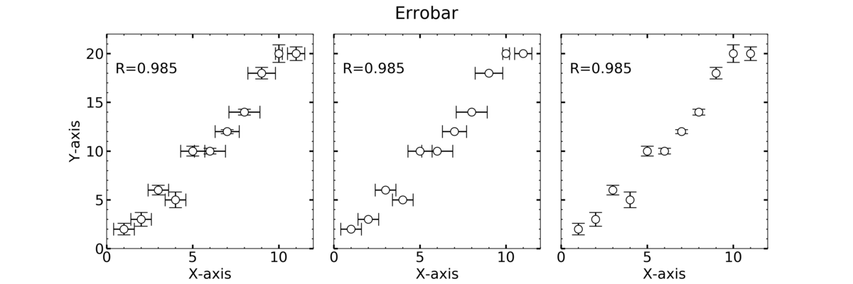
plt.suptitle("Errobar")
ax1 = plt.subplot(131)
ax2 = plt.subplot(132)
ax3 = plt.subplot(133)
ax1.errorbar(x, y, xerr=x_err, yerr=y_err, fmt = "o"
,markersize = 10,color="k", markerfacecolor="w",capsize=8)
ax2.errorbar(x, y, xerr=x_err, fmt = "o"
,markersize = 10,color="k", markerfacecolor="w",capsize=8)
ax3.errorbar(x, y, yerr=y_err, fmt = "o"
,markersize = 10,color="k", markerfacecolor="w",capsize=8)
axes = [ax1, ax2, ax3]
for ax in axes:
#範囲の設定
ax.set_xlim(0, 12)
ax.set_ylim(0, 22)
#メモリの設定
ax.minorticks_on() #補助メモリの描写
ax.tick_params(axis="both", which="major",direction="in",length=5,width=2,top="on",right="on")
ax.tick_params(axis="both", which="minor",direction="in",length=2,width=1,top="on",right="on")
#ラベルの設定
ax.set_xlabel("X-axis")
ax.set_ylabel("Y-axis")
#テキストの貼り付け
ax.text(0.5, 18, "R={:.3f}".format(corr[0,1]))
ax.label_outer()
plt.subplots_adjust(wspace=0.1)
plt.show()
#保存
fig.savefig("XXX.png",format="png", dpi=330)
回帰直線
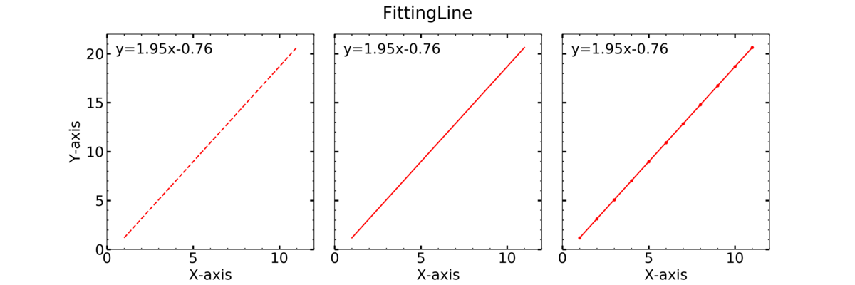
1次の回帰なので、y=ax+bが求める回帰直線です。 以下の操作で計算できます。
#回帰直線
p = np.polyfit(x, y, 1)
y_reg = x*p[0]+p[1]
np.polyfit(xのデータ, yのデータ, 次元)
p[0]=傾き
p[1]=切片
グラフ作成
グラフを書いてみます。
fig = plt.figure(figsize=(15,5))
plt.rcParams["font.size"] = 18
plt.suptitle("FittingLine")

ax1 = plt.subplot(131)
ax2 = plt.subplot(132)
ax3 = plt.subplot(133)

ax1.plot(x, y_reg, "--" ,color="r")
ax2.plot(x, y_reg, "-" ,color="r")
ax3.plot(x, y_reg, ".-" ,color="r")

axes = [ax1, ax2, ax3]
for ax in axes:
    #範囲の設定
    ax.set_xlim(0, 12)
    ax.set_ylim(0, 22)

    #メモリの設定
    ax.minorticks_on() #補助メモリの描写
    ax.tick_params(axis="both", which="major",direction="in",length=5,width=2,top="on",right="on")
    ax.tick_params(axis="both", which="minor",direction="in",length=2,width=1,top="on",right="on")

    #ラベルの設定
    ax.set_xlabel("X-axis")
    ax.set_ylabel("Y-axis")

    #テキストの貼り付け
    ax.text(0.5, 20, "y={:.2f}".format(p[0])+"x{0:+.2f}".format(p[1]))

    ax.label_outer()

plt.subplots_adjust(wspace=0.1)
plt.show()

#保存
fig.savefig("XXX.png",format="png", dpi=330)
相関グラフまとめ
def main():
    fig = plt.figure(figsize=(10,10))
    plt.rcParams["font.size"] = 18

    ax = plt.subplot(111)

    ax.errorbar(x, y, xerr=x_err, yerr=y_err, fmt = "o"
                 ,markersize = 10,color="k", markerfacecolor="w",capsize=8)
    ax.plot(x, y_reg, color="r")

    #範囲の設定
    ax.set_xlim(0, 12)
    ax.set_ylim(0, 22)

    #メモリの設定
    ax.minorticks_on() #補助メモリの描写
    ax.tick_params(axis="both", which="major",direction="in",length=5,width=2,top="on",right="on")
    ax.tick_params(axis="both", which="minor",direction="in",length=2,width=1,top="on",right="on")

    #ラベルの設定
    ax.set_title("Correlation")
    ax.set_xlabel("X-axis")
    ax.set_ylabel("Y-axis")

    #テキストの貼り付け
    ax.text(0.5, 20, "y={:.2f}".format(p[0])+"x{0:+.2f}".format(p[1]))
    ax.text(0.5, 18, "R={:.3f}".format(corr[0,1]))

    plt.show()

    #保存
    fig.savefig("XXX.png",format="png", dpi=330)

if __name__ == "__main__":
    main()

参考
それでは 🌏